A primer into Risk Management with R. Analyzing VaR and CVaR with Monte Carlo Simulations

Introduction

Risk management is a crucial aspect of financial modeling, and one of the key metrics used to measure risk is Value at Risk (VaR). In this project, we explore different approaches to computing VaR, including Historical VaR, Parametric VaR, and Cornish-Fisher VaR, as well as Conditional VaR (CVaR). Additionally, we compare these risk measures across different shock distributions using Monte Carlo simulations.

Step 1: Simulating Historical Price Data

To analyze risk, we first generate synthetic historical price data using a Geometric Brownian Motion (GBM) model with normal shocks. The resulting price series is converted into an xts object for time series analysis.

# Generating synthetic historical data from a GBM with normal shocks
historical_data <- simulate_gbm_with_shocks(S0 = 100, drift = 0.05, sigma = 0.2, T = 1, N = 252, distribution = "std_normal")

# Convert to xts object
dates <- seq(as.Date("2023-01-01"), by = "day", length.out = 253)
historical_xts <- xts(historical_data, order.by = dates)

Step 2: Computing Historical VaR

Historical VaR is calculated by analyzing the empirical distribution of daily log returns.

returns <- diff(log(historical_xts))[-1]
VaR_95 <- quantile(returns, probs = 0.05)
VaR_99 <- quantile(returns, probs = 0.01)

Step 3: Parametric VaR

Parametric VaR assumes that returns follow a normal distribution, allowing us to use the mean and standard deviation to estimate risk.

mean_return <- mean(returns)
sd_return <- sd(returns)
parametric_VaR_95 <- mean_return + sd_return * qnorm(0.05)
parametric_VaR_99 <- mean_return + sd_return * qnorm(0.01)

Step 4: Computing CVaR (Expected Shortfall)

Conditional VaR (CVaR) provides an expectation of losses beyond the VaR threshold.

CVaR_95 <- mean(returns[returns <= VaR_95])
CVaR_99 <- mean(returns[returns <= VaR_99])

Step 5: Cornish-Fisher Expansion

The Cornish-Fisher expansion adjusts VaR estimates by incorporating skewness and kurtosis.

skewness <- PerformanceAnalytics::skewness(returns)
kurtosis <- PerformanceAnalytics::kurtosis(returns)

z_95 <- qnorm(0.05)
z_99 <- qnorm(0.01)

adjusted_z_95 <- z_95 + (skewness / 6) * (z_95^2 - 1) + (kurtosis / 24) * (z_95^3 - 3 * z_95)
CF_VaR_95 <- mean_return + sd_return * adjusted_z_95

Step 6: Scenario Analysis Across Different Distributions

We expand our analysis by simulating returns from different shock distributions:

• Standard Normal
• Skewed Normal
• Heavy-Tailed Normal
• t-Distribution
• Skewed t-Distribution

Each scenario is analyzed using the same risk measures.

scenarios <- list(
  list(distribution = "std_normal"),
  list(distribution = "skewed_normal", alpha = 5),
  list(distribution = "heavy_tail_normal", df = 3),
  list(distribution = "std_t", df = 5)
)
results_list <- map(scenarios, ~ do.call(analyze_shock_scenario, .))
results_df <- bind_rows(results_list)

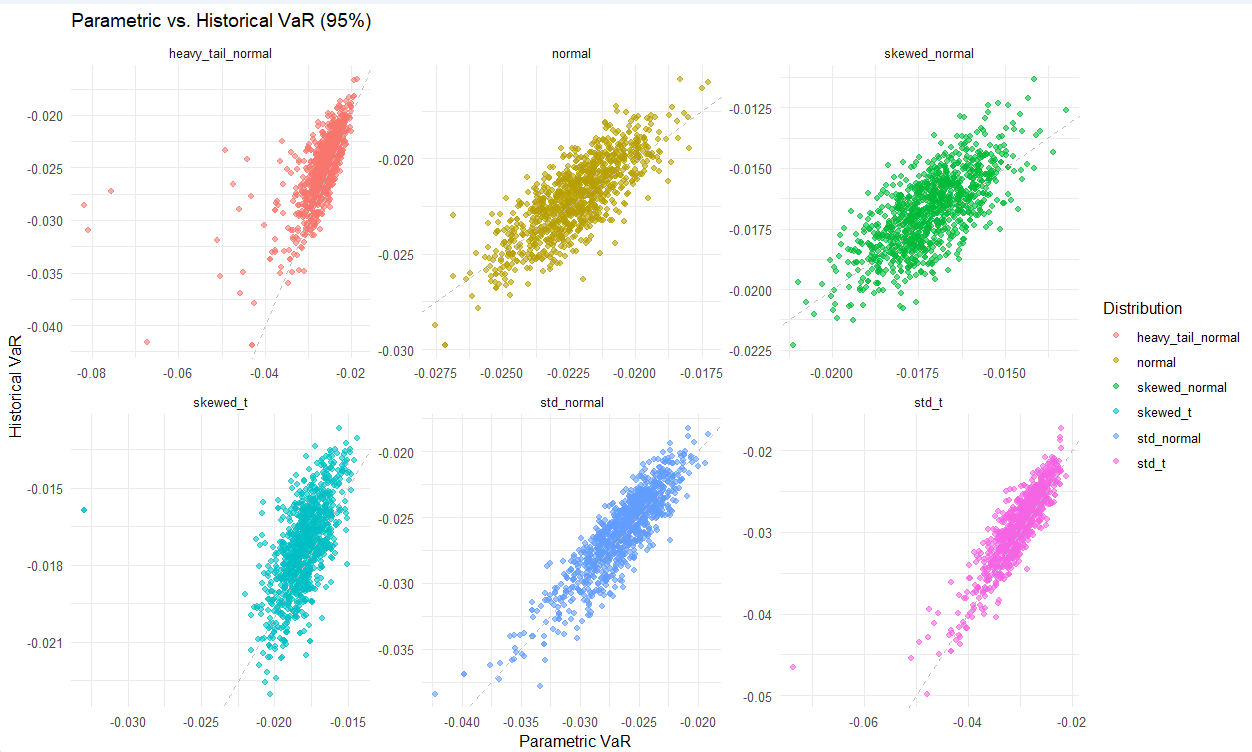
Step 7: Monte Carlo Simulations

We run 1,000 Monte Carlo simulations to test the robustness of our risk measures across different distributions.

monte_carlo_results <- future_map(1:1000, ~ {
  map(scenarios, ~ do.call(analyze_shock_scenario, c(., seed = runif(n = 1)*1000000)))
}, .progress = TRUE)

Step 8: Visualizing Results

We use ggplot2 to visualize the comparison of different risk measures.

ggplot(results_df, aes(x = Distribution, y = Value, fill = Metric)) +
  geom_bar(stat = "identity", position = "dodge") +
  labs(title = "Comparison of Risk Measures", x = "Shock Distribution", y = "Value") +
  theme_minimal()

Conclusion

This project demonstrates how to systematically analyze financial risk using different VaR methodologies and Monte Carlo simulations. By incorporating various shock distributions, we gain deeper insights into the robustness of risk metrics under different market conditions.