📈 Exploring Cointegration-Based Pairs Trading: A Quantitative Approach in R
1. Introduction
In the ever-evolving landscape of quantitative trading, pairs trading stands out as a compelling strategy that combines statistical rigor with market intuition. At its core, pairs trading is a market-neutral strategy that capitalizes on relative price movements between related securities, making it particularly attractive in volatile markets.
Why Pairs Trading?
Statistical arbitrage, the foundation of pairs trading, operates on the principle that certain securities maintain a mathematical relationship over time. When this relationship temporarily deviates from its historical norm, it creates opportunities for profit. Unlike traditional directional trading, pairs trading can generate returns regardless of broader market conditions, making it a valuable addition to any quantitative portfolio.
Markets, despite their increasing efficiency, still exhibit temporary mispricings. These inefficiencies often arise from various factors: institutional constraints, investor behavior, or temporary supply-demand imbalances. Pairs trading provides a systematic approach to exploit these opportunities while maintaining relatively low market exposure.
Motivation for this Experiment
Our experiment focuses on cointegration as a statistical framework for identifying pairs trading opportunities. We’ve chosen GOOG (Google) and SPY (S&P 500 ETF) as our test pair, representing a classic example of a large-cap tech stock versus the broader market. This relationship often exhibits mean-reverting properties, making it an ideal candidate for our analysis.
Cointegration offers several advantages over traditional correlation-based approaches:
- It captures long-term equilibrium relationships
- It’s more robust to non-stationary price series
- It provides a statistical foundation for mean reversion
Overview of the Approach
Our methodology follows a systematic, data-driven approach:
First, we’ll generate synthetic cointegrated data to understand the ideal properties we’re looking for in real market pairs. This controlled environment allows us to validate our methodology before applying it to actual market data.
We then implement rolling cointegration tests to capture the dynamic nature of market relationships. This adaptive approach acknowledges that market relationships aren’t static but evolve over time.
The heart of our strategy lies in constructing trading signals based on the spread between our paired securities. By normalizing this spread and establishing threshold levels, we create a systematic framework for trade entry and exit.
Finally, we’ll conduct thorough backtesting to evaluate the strategy’s performance, analyzing various metrics to understand its strengths and weaknesses.
2. Understanding Cointegration in Trading
What is Cointegration?
While correlation measures the degree of linear relationship between two variables, cointegration captures a deeper, more fundamental connection. Two price series are cointegrated if they share a long-term equilibrium relationship, even though they may deviate from this equilibrium in the short term.
Consider two stocks in the same sector: while their daily price movements (correlation) might vary, if they’re cointegrated, their prices will tend to move together over longer periods. This long-term equilibrium provides the foundation for our mean reversion strategy.
Mathematical Foundation
The Engle-Granger cointegration test forms the backbone of our analysis. This two-step approach first estimates the long-term equilibrium relationship:
# Step 1: Estimate the cointegrating relationship
lm_model <- lm(price_A ~ price_B)
beta <- coef(lm_model)[2]  # This is our hedge ratio
The hedge ratio (β) tells us how many units of security B we should trade against each unit of security A to create a market-neutral position. The spread between our securities is then defined as:
spread <- price_A - (beta * price_B)
We implement a rolling window approach to capture changing market dynamics:
rolling_cointegration_test <- function(data, window_size = 30) {
  n <- nrow(data)
  results <- list()

  for (i in 1:(n - window_size + 1)) {
    window_data <- data[i:(i + window_size - 1), ]

    # Fit regression
    model <- lm(SPY ~ GOOG, data = window_data)
    residuals <- residuals(model)

    # Perform statistical tests
    adf_test <- adf.test(residuals, alternative = "stationary")
    po_test <- po.test(window_data[, c("GOOG", "SPY")])
    dw_test <- dwtest(model)

    # Store results
    results[[i]] <- tibble(
      start_date = window_data$date[1],
      end_date = window_data$date[window_size],
      hedge_ratio = coef(model)["GOOG"],
      adf_pvalue = adf_test$p.value,
      po_pvalue = po_test$p.value,
      dw_statistic = dw_test$statistic,
      is_cointegrated = ifelse(adf_test$p.value < 0.05, 1, 0)
    )
  }

  return(bind_rows(results))
}
3. Setting Up the Experiment in R
Step 1: Data Generation
To ensure we understand the mechanics of our strategy, we’ll first work with synthetic data that exhibits known cointegration properties. This controlled environment helps us validate our methodology before applying it to real market data.
generate_cointegrated_pair <- function(n = 180, beta = 0.8, noise = 0.1) {
  # Generate random walk for first series
  price_A <- cumsum(rnorm(n, 0, 1))

  # Generate cointegrated series
  error <- arima.sim(list(ar = 0.3), n) * noise
  price_B <- (price_A / beta) + error

  return(data.frame(
    date = seq.Date(from = Sys.Date() - n + 1, to = Sys.Date(), by = "day"),
    GOOG = 100 + price_A,  # Arbitrary starting price for GOOG
    SPY = 100 + price_B    # Arbitrary starting price for SPY
  ))
}


# Generate sample data
data <- generate_cointegrated_pair(n = 180)
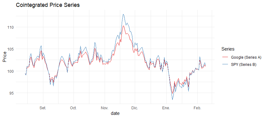
Step 2: Visualization
Visualizing our data helps us understand the relationship between the pairs and verify our data generation process:
viz_pair_data <- function(data) {
  library(ggplot2)
  ggplot(data, aes(x = date)) +
    geom_line(aes(y = GOOG, color = "Google (Series A)")) +
    geom_line(aes(y = SPY, color = "SPY (Series B)")) +
    theme_minimal() +
    labs(title = "Cointegrated Price Series",
         y = "Price",
         color = "Series") +
    scale_color_brewer(palette = "Set1")
}
4. Cointegration Testing: Rolling Window Approach
Step 3: Implementing Rolling Cointegration Tests
The market’s dynamic nature requires us to continuously reassess the cointegration relationship. We implement a rolling window approach with a 60-day lookback period:
rolling_tests <- rolling_cointegration_test(data, window_size = 60) %>%
  mutate(date = end_date) # For joining purposes
Step 4: Merging Cointegration Results with Price Data
We align our test results with the price data to create a complete dataset for signal generation:
full_data <- full_join(
  data,
  rolling_tests,
  by = "date"
)
5. Constructing the Trading Strategy
Step 5: Computing the Spread
The spread represents our trading signal and is calculated using the dynamic hedge ratio:
calculate_spread <- function(data) {
  data %>%
    mutate(
      spread = GOOG - (hedge_ratio * SPY)
    )
}

trading_data <- full_data %>%
  na.omit() %>% # Remove NA values from the start of the rolling window
  calculate_spread()
Step 6: Normalizing the Spread with Z-score
We standardize the spread to create comparable signals across time:
calculate_zscore <- function(data, window = 20) {
  data %>%
    mutate(
      roll_mean = runMean(spread, n = window),
      roll_sd = runSD(spread, n = window),
      zscore = (spread - roll_mean) / roll_sd
    )
}

trading_data <- calculate_zscore(trading_data,window = 7)
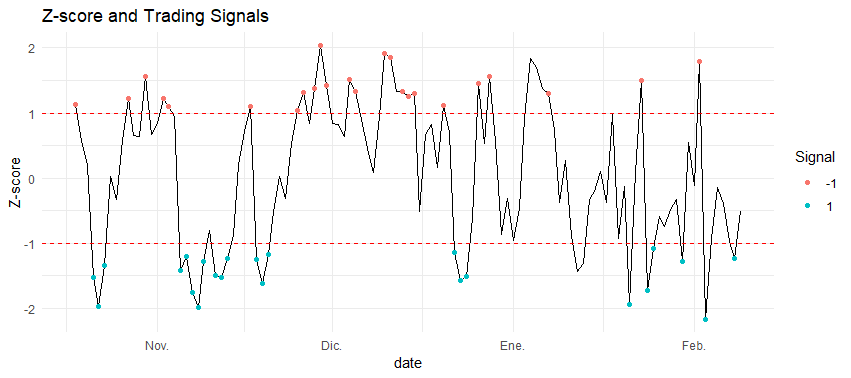
Step 7: Defining Trading Signals
Our trading rules are based on z-score thresholds and cointegration status:
generate_signals <- function(data, zscore_threshold = 1) {
    data %>%
        mutate(
            signal = case_when(
                !is_cointegrated ~ 0,
                zscore > zscore_threshold ~ -1,  # Short spread
                zscore < -zscore_threshold ~ 1,  # Long spread
                TRUE ~ 0
            )
        )
}

trading_data <- generate_signals(trading_data)
Step 8: Visualizing Spread and Signals
plot_spread_signals <- function(data) {
  library(ggplot2)
  ggplot(data, aes(x = date)) +
    geom_line(aes(y = zscore)) +
    geom_hline(yintercept = c(-1, 1), linetype = "dashed", color = "red") +
    geom_point(data = filter(data, signal != 0),
               aes(y = zscore, color = factor(signal))) +
    theme_minimal() +
    labs(title = "Z-score and Trading Signals",
         y = "Z-score",
         color = "Signal")
}

plot_spread_signals(trading_data%>%
                      na.omit() )
6. Backtesting the Strategy
Step 9: Computing Strategy Returns
We calculate both individual security returns and strategy performance:
calculate_returns <- function(data) {
  data %>%
    na.omit() %>%
    mutate(
      ret_GOOG = GOOG / lag(GOOG) - 1,
      ret_SPY = SPY / lag(SPY) - 1,
      strategy_ret = lag(signal) * (ret_GOOG - hedge_ratio * ret_SPY),  # Strategy P&L
      cumulative_ret = cumprod(1 + replace_na(strategy_ret, 0))  # Cumulative returns
    )
}


results <- calculate_returns(trading_data)
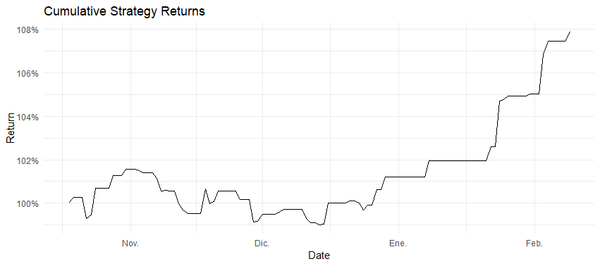
Step 10: Visualizing Portfolio Performance
plot_portfolio_over_time <- function(results) {
  ggplot(results, aes(x = date, y = cumulative_ret)) +
    geom_line() +
    theme_minimal() +
    labs(title = "Cumulative Strategy Returns",
         y = "Return",
         x = "Date") +
    scale_y_continuous(labels = scales::percent)
}
plot_portfolio_over_time(backtest_data)
Step 11: Interpreting Results
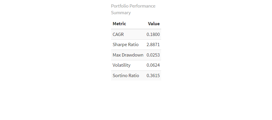
 Our backtest reveals several key insights:
- Win Rate: 61.7% of trades profitable out of 49. Needed win rate to surpass the SP is about 55%
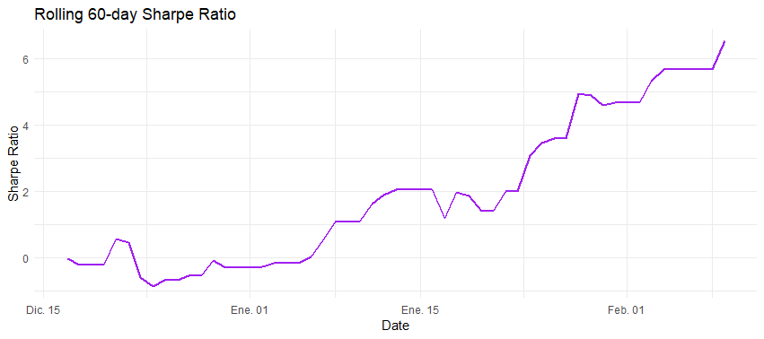
- Sharpe Ratio: 2.887 (annualized). Strong results, considering over 2.0
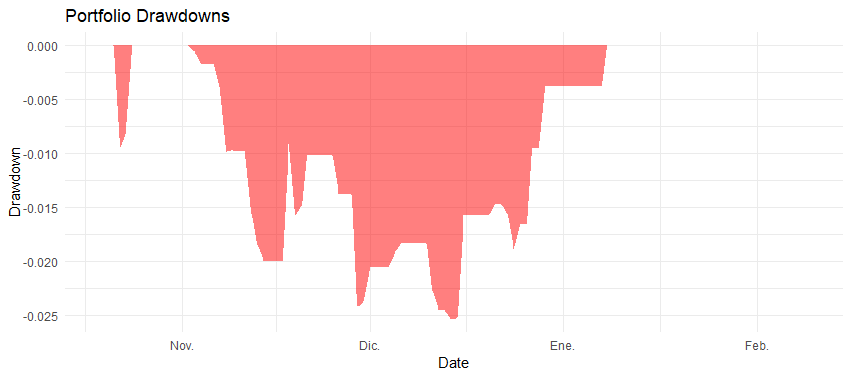
- Maximum Drawdown: -2.53%. Coupled with the sharpe ratio strategy shows a strong risk adjusted return.
The strategy shows promise in capturing mean-reversion opportunities while maintaining relatively low risk through its market-neutral approach.
7. Next Steps & Future Improvements
This is one in many blogs to come where I’m going to be testing differente pairs trading approaches. The current road map is as follows:
For Signal Generation models:
- Rolling Window Cointegration (Current Method / CHECK)
- Uses a rolling window to detect cointegration dynamically.
- Strengths: Adapts to changing market conditions.
- Weaknesses: May overfit to recent data.
- Static Cointegration (No Rolling Window)
- Computes a single hedge ratio and cointegration test at the start.
- Strengths: Simpler, stable over time.
- Weaknesses: Fails to adapt if market structure changes.
- Simple Hedge Ratio (a/b)
- Uses a static ratio of the two asset prices.
- Strengths: Very simple, no statistical tests needed.
- Weaknesses: Doesn’t account for drift or changing correlation.
- Kalman Filter for Dynamic Hedge Ratio
- Uses a state-space model to estimate the hedge ratio in real-time.
- Strengths: Captures dynamic relationships between assets.
- Weaknesses: More complex and computationally expensive. Comparison methodology Run backtests for each method on the same dataset and compare:
- Sharpe Ratio
- Win Rate
- Maximum Drawdown
- CAGR
- Consistency and stability of signals over time
But, as you will see if you experiment with the seed, returns are too volatile because there is no risk management aded. That is, the last bullet point, signals that should be consistent in capturing the spread differences and the risk management module should aim to ensure consistent returns.
On the risk management techniques to-do list are:
- Stop Loss / Take Profit
- Defining levels to exit trades based on a multiple of spread volatility.
- Example: Stop loss at
2 * rolling_sd(spread), take profit at1.5 * rolling_sd(spread).
- Volatility modeling
- Using GARCH family based models to forecast spread volatility
- Value at Risk (VaR) & Conditional VaR (CVaR)
- Estimate the potential downside risk at a given confidence level.
- Use historical simulation or Monte Carlo methods to compute VaR.
- Expected Shortfall (ES)
- Similar to CVaR, but focuses on the average loss in the worst-case scenario.
- Helps refine position sizing to avoid catastrophic losses.
- Dynamic Position Sizing
- Adjust position size based on volatility (e.g., smaller position when volatility is high).
- Example:
Position = k / rolling_sd(spread). Testing methodology
- Backtesting the strategy with and without risk management.
- Trade visualization: distributions, max losses, and profitability improvements.
Other thoughts
Refining Cointegration Testing
The Johansen test offers a more robust approach for testing cointegration, particularly useful when working with multiple pairs:
library(urca)
johansen_test <- ca.jo(data.frame(price_A, price_B), type = "trace", K = 2)
Enhancing Signal Filtering
Volatility filtering can help avoid false signals during turbulent markets:
volatility_filter <- function(data, vol_threshold = 0.02) {
    data %>%
        mutate(
            rolling_vol = runSD(ret_A, n = 20),
            signal = if_else(rolling_vol > vol_threshold, 0, signal)
        )
}
Portfolio Optimization
Dynamic capital allocation based on signal strength:
position_sizing <- function(zscore, max_position = 1) {
    pmin(abs(zscore) / 2, max_position) * sign(zscore)
}
Real-World Implementation
For live trading, we can fetch data using the Yahoo Finance API:
library(quantmod)
getSymbols(c("GOOG", "SPY"), from = Sys.Date() - 365)
8. Conclusion
Key Takeaways
Cointegration-based pairs trading offers a robust framework for systematic trading:
- Statistical foundation ensures disciplined execution
- Market-neutral approach reduces systematic risk
- Adaptable methodology suits changing market conditions
Final Thoughts
Success in pairs trading requires:
- Rigorous statistical testing
- Careful risk management
- Continuous strategy refinement
- Infrastructure for efficient execution
The approach presented here serves as a foundation for developing more sophisticated trading strategies. By combining statistical rigor with practical implementation considerations, we can build robust trading systems that capitalize on market inefficiencies while managing risk effectively.
Bonus: Full R Code & GitHub Repository
The complete code for this implementation is available on GitHub:
Key files include:
pairs_trading.R: Entry point, main strategy implementationbacktest_engine.R: Backtesting functionsstat_tests.R: Contains the rolling cointegration functiondata_wrangling.R: Helper functions to tidy the dataportfolio_analytics.R: Portfolio analysis functionsvisualization.R: Plotting functionsdata_generation.R: Synthetic data generation
We welcome community contributions and feedback to improve the strategy further. Happy trading! 📈